

Summary
This article offers a comprehensive guide on understanding football match dynamics through statistical event data, crucial for coaches, analysts, and fans alike. Key Points:
- Delve into advanced methodologies for calculating expected threat (xT) and player value (PV), addressing their limitations and biases stemming from different models and datasets.
- Explore dynamic threshold determination methods that consider factors like opponent strength and game stage, utilizing machine learning to personalize performance metrics for players and teams.
- Compare various time window and decay function strategies to optimize performance analysis, showcasing real-world examples of how these approaches impact momentum shifts.

In this article, I will guide you through the process of calculating match momentum using event data. We will focus on the Expected Threat (xT) metric—if you're not familiar with xT, there's no need to worry; I'll explain it along the way. Our methodology will be based on insights from Opta Analyst, a well-known name in football analytics. If you've ever explored this field, you're likely familiar with their captivating match momentum visuals. As I mentioned in my previous post, we will utilize free StatsBomb match event data. By the end of this article, you'll find a Python function that you can easily copy and incorporate into your own projects.
Key Points Summary
- Event data refers to time-stamped information that captures significant occurrences in a system or application.
- It plays a crucial role in event-driven architectures and is essential for understanding user behavior and traffic patterns.
- Businesses utilize event data to gain insights, improve decision-making, and enhance customer experiences.
- Event data can be collected through various tracking tools, providing valuable metrics for analysis.
- Data accuracy and security are emphasized when managing event data for businesses` analytics needs.
- The Event Data API offers raw details about events along with contextual information about their collection.
In our fast-paced digital world, understanding what happens within our systems is more important than ever. From tracking user behaviors to optimizing business decisions, event data is like a behind-the-scenes look at the actions that shape our experiences. By collecting this information accurately and securely, businesses can truly connect with their users and create better services tailored to their needs.
Extended Comparison:| Event Data Source | Key Features | Use Cases | Trends | Security Measures |
|---|---|---|---|---|
| Google Analytics 4 | Real-time tracking, user-centric data model | Website traffic analysis, user engagement insights | Increased focus on privacy and consent management | Enhanced encryption protocols for data in transit |
| Mixpanel | Event-based analytics, cohort analysis tools | Product usage tracking, funnel analysis | Shift towards mobile-first analytics solutions | Robust access controls and data encryption |
| Amplitude | Behavioral cohorting, powerful segmentation tools | Customer journey mapping, retention strategies | Integration of machine learning for predictive analytics | Regular security audits and compliance with GDPR |
| Heap Analytics | Automatic event tracking, retroactive analysis capabilities | Conversion optimization, A/B testing support | Rise in automated insights generation via AI | Data anonymization techniques to protect user identity |
| Hotjar | Heatmaps, session recordings for UX improvements | User experience evaluation, feedback collection | Growing emphasis on integrated customer feedback loops | Strict GDPR compliance measures |
To begin with, let's explore how Opta examines the concept of match momentum. For those interested in a more comprehensive understanding, their complete article is available for reading, but for now, we’ll focus on an overview of their methodology.

Opta meticulously breaks down each match minute by minute, evaluating the most threatening attempts made by both teams in terms of their likelihood to lead to a goal. Notably, actions that occur later in the game carry more weight in this assessment. As you may have noticed, Opta frequently references a concept known as possession value. This framework defines possession value (PV) as a measure of the probability that the team currently holding the ball will score within the next 10 seconds, allowing for an analysis of individual players' contributions—both positive and negative—during play.
Quantifying Scoring Potential: Unveiling the Power of Expected Threat (xT) and Player Value (PV)
The understanding of player performance and scoring potential in soccer has evolved significantly, particularly with the introduction of advanced metrics. One key metric is the Expected Threat (xT), which quantifies the likelihood of a goal being scored from specific areas on the pitch. By segmenting the field into various zones, each assigned a value based on its distance to the goal, teams can gain insights into where offensive plays are most likely to result in scoring opportunities.In addition to xT, Player Value (PV) serves as another essential measure that captures an individual player's impact on their team's scoring chances. This metric evaluates how a player's movements alter the xT by comparing values from zones they enter and exit while in possession of the ball. A higher difference indicates a greater contribution to enhancing their team's probability of scoring.
Together, these metrics provide a comprehensive view of both team dynamics and individual performances, allowing coaches and analysts to make more informed decisions regarding strategies and player roles.

The document featuring the same grid as shown above can be found here. Let's delve deeper into Opta's methodology. While we won't strictly adhere to their methods, there are several important aspects that deserve our attention.
Why is it beneficial to focus solely on the highest expected threat (xT) value from each segment? Consider a scenario where one team methodically builds their attack, completing numerous passes just outside the opponent's penalty area. After an extended sequence of these passes, the opposing team regains possession and launches a rapid counter-attack, transitioning the ball quickly from one end of the field to the other. While the total xT accumulated from all those passes by the first team might surpass that of a single carry by their rivals, this does not necessarily indicate that they posed a greater threat overall.
Contextual Threshold Determination for Accurate Player Performance Evaluation in Sports Analytics
In sports analytics, particularly in evaluating player performance through expected goals (xG) or expected assists (xA), it is crucial to establish an appropriate clipping threshold for xT values. The determination of this threshold should be context-sensitive and aligned with the distribution of the data at hand. An excessively low threshold may fail to mitigate inflated xT values effectively, while a very high threshold could inadvertently eliminate important insights that contribute to understanding player contributions.To enhance accuracy and relevance in analysis, implementing a dynamic clipping algorithm can be beneficial. This approach allows for adjustments based on various factors, including game context, team dynamics, and individual player skills. Such tailored methods can lead to more precise evaluations and better decision-making processes within coaching staff and analysts.
from statsbombpy import sb sb.competitions().query('competition_name == "La Liga" & season_name == "2018/2019"')
sb.matches(competition_id=11, season_id=4).query('home_team == "Espanyol"')
Now that we have acquired the necessary ID values, we can proceed to retrieve the match event data.
MATCH_ID = 16086 HOME_TEAM, AWAY_TEAM = 'Espanyol', 'Barcelona' df = sb.events(match_id=MATCH_ID)The initial step involves importing values from our xT model, along with essential libraries. You can find the Expected Threat grid file in one of my GitHub repositories here.
import pandas as pd import numpy as np xT = pd.read_csv("https://raw.githubusercontent.com/AKapich/WorldCup_App/main/app/xT_Grid.csv", header=None) xT = np.array(xT) xT_rows, xT_cols = xT.shapeAmong all match events, our focus is solely on passes and carries, as these actions involve the movement of the ball across different areas of the pitch. In our dataset, we have specific columns for location, pass_end_location, and carry_end_location, which will aid us in calculating expected threat (xT) for each action. Below, I will present a universal function designed for this calculation and illustrate it with an example involving player passes. Subsequently, we will utilize this function to derive xT from both passes and carries and combine our findings into a cohesive result.
def get_xT(df, event_type): df = df[df['type']==event_type] df['x'], df['y'] = zip(*df['location']) df['end_x'], df['end_y'] = zip(*df[f'{event_type.lower()}_end_location']) df[f'start_x_bin'] = pd.cut(df['x'], bins=xT_cols, labels=False) df[f'start_y_bin'] = pd.cut(df['y'], bins=xT_rows, labels=False) df[f'end_x_bin'] = pd.cut(df['end_x'], bins=xT_cols, labels=False) df[f'end_y_bin'] = pd.cut(df['end_x'], bins=xT_rows, labels=False) df['start_zone_value'] = df[[f'start_x_bin', f'start_y_bin']].apply(lambda z: xT[z[1]][z[0]], axis=1) df['end_zone_value'] = df[[f'end_x_bin', f'end_y_bin']].apply(lambda z: xT[z[1]][z[0]], axis=1) df['xT'] = df['end_zone_value']-df['start_zone_value'] return df[['xT', 'minute', 'second', 'team', 'type']]Let's create an auxiliary data frame so that you can analyze better what the function does. It will contain only passes (as if we gave 'Pass' as an argument to the function).
from copy import deepcopy aux_df = deepcopy(df) aux_df = aux_df[aux_df['type']=='Pass']Each row includes coordinate information.

We are going to analyze and categorize the values, identifying the areas from which passes began and where they ended. This will entail dividing the pitch into specific zones that correspond with our analytical framework.
aux_df['x'], aux_df['y'] = zip(*aux_df['location']) aux_df['end_x'], aux_df['end_y'] = zip(*aux_df[f'pass_end_location']) aux_df[f'start_x_bin'] = pd.cut(aux_df['x'], bins=xT_cols, labels=False) aux_df[f'start_y_bin'] = pd.cut(aux_df['y'], bins=xT_rows, labels=False) aux_df[f'end_x_bin'] = pd.cut(aux_df['end_x'], bins=xT_cols, labels=False) aux_df[f'end_y_bin'] = pd.cut(aux_df['end_x'], bins=xT_rows, labels=False)Now rather than utilizing specific coordinates, we are focusing on defined areas of the pitch.

By understanding the various zones, we can now allocate expected threat (xT) values to each area and determine the difference in xT between the starting zone and the end zone.
aux_df['start_zone_value'] = aux_df[[f'start_x_bin', f'start_y_bin']].apply(lambda z: xT[z[1]][z[0]], axis=1) aux_df['end_zone_value'] = aux_df[[f'end_x_bin', f'end_y_bin']].apply(lambda z: xT[z[1]][z[0]], axis=1) aux_df['xT'] = aux_df['end_zone_value']-aux_df['start_zone_value']
As you’re already familiar with how we calculate the expected threat (xT) for each action, we can proceed to the next phase. The following step involves merging our xT values derived from both passes and carries, followed by applying a clipping process. For this task, I plan to utilize a cap value of 0.1, consistent with the approach taken by Opta.
xT_data = pd.concat([get_xT(df=df, event_type='Pass'), get_xT(df=df, event_type='Carry')], axis=0) xT_data['xT_clipped'] = np.clip(xT_data['xT'], 0, 0.1)Now, it's time to find the maximum xT values each team obtained minute by minute.
max_xT_per_minute = xT_data.groupby(['team', 'minute'])['xT_clipped'].max().reset_index()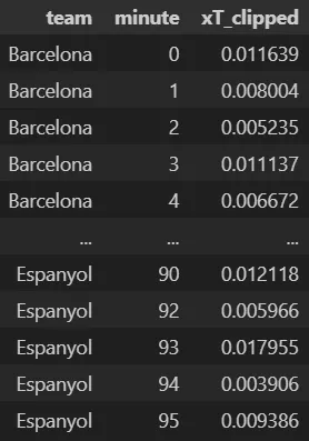
Time Window and Decay Function Optimization in Sports Performance Analysis
When analyzing sports performance and outcomes, it is crucial to determine an optimal time window for data collection. This window should be tailored to each specific sport and its unique match dynamics, as well as the availability of relevant data. For instance, in fast-paced sports such as soccer or basketball, a time window of 3-5 minutes may be appropriate to capture critical moments without losing detail. Conversely, for slower-paced games like baseball or cricket, extending this period to 5-10 minutes can provide a clearer picture of player actions and strategies over time.Additionally, selecting the right decay function is vital in modeling past performance influences accurately. While exponential decay is frequently employed due to its effectiveness in illustrating how past actions gradually lose relevance over time, other functions such as linear or logarithmic decay might also serve well depending on the context. The key lies in fine-tuning the decay rate to balance immediate performance trends with historical consistency while preventing older actions from disproportionately skewing current evaluations.
In the provided code, we examine each minute of the game, focusing solely on those that fall within a specified timeframe. We then apply an exponential function to calculate weights, ultimately aggregating these values for each team. The momentum at any given minute is determined by the disparity in weighted xT values between the two teams.
The exponential function is particularly well-suited for modeling weights in our scenario. It's important to note that the decay rate is expressed as a negative value. When you examine the behavior of the exponential function with negative inputs, you'll find that smaller input values yield even smaller outputs. This is why a larger decay rate emphasizes more recent occurrences — by using -1 to multiply, we introduce a negative argument into the function, resulting in diminished weights for events that occurred only minutes ago.
minutes = sorted(xT_data['minute'].unique()) weighted_xT_sum = { HOME_TEAM: [], AWAY_TEAM: [] } momentum = [] window_size = 4 decay_rate = 0.25 for current_minute in minutes: for team in weighted_xT_sum.keys(): recent_xT_values = max_xT_per_minute[ (max_xT_per_minute['team'] == team) & (max_xT_per_minute['minute'] <= current_minute) & (max_xT_per_minute['minute'] > current_minute - window_size) ] weights = np.exp(-decay_rate * (current_minute - recent_xT_values['minute'].values)) weighted_sum = np.sum(weights * recent_xT_values['xT_clipped'].values) weighted_xT_sum[team].append(weighted_sum) momentum.append(weighted_xT_sum[HOME_TEAM][-1] - weighted_xT_sum[AWAY_TEAM][-1]) momentum_df = pd.DataFrame({ 'minute': minutes, 'momentum': momentum })In conclusion, we've created a data frame that captures the momentum of each match on a minute-by-minute basis. Positive figures reflect the home team's control over the game, while negative numbers signify that the away team is taking charge.

The most critical part of our analysis is already behind us; what remains now is to craft a visually appealing representation of the data. To begin, we will focus on plotting the momentum curve. Our primary interest lies not in the precise values, but rather in identifying which team exhibits greater dominance. To achieve this, we'll need to smooth out our curve. We can do this by applying a Gaussian filter to our data. In essence, a Gaussian filter alters the input data through convolution with a Gaussian function. By adjusting the sigma parameter, we can control the level of smoothness—higher sigma values yield a smoother curve.
In the following code, I ensure that various aesthetic aspects are taken into account. The plot's frame is eliminated, ticks on the x-axis are set to appear every 15 minutes, and unnecessary margins are removed.
import matplotlib.pyplot as plt from scipy.ndimage import gaussian_filter1d fig, ax = plt.subplots(figsize=(12, 6)) fig.set_facecolor('#0e1117') ax.set_facecolor('#0e1117') ax.tick_params(axis='x', colors='white') ax.margins(x=0) ax.set_xticks([0,15,30,45,60,75,90]) ax.tick_params(axis='y', which='both', left=False, right=False, labelleft=False) ax.set_ylim(-0.08, 0.08) for spine in ['top', 'right', 'bottom', 'left']: ax.spines[spine].set_visible(False) momentum_df['smoothed_momentum'] = gaussian_filter1d(momentum_df['momentum'], sigma=1) ax.plot(momentum_df['minute'], momentum_df['smoothed_momentum'], color='white')
Next, we wish to apply the distinctive colors indicating which team currently controls the match.
ax.axhline(0, color='white', linestyle='--', linewidth=0.5) ax.fill_between(momentum_df['minute'], momentum_df['smoothed_momentum'], where=(momentum_df['smoothed_momentum'] > 0), color='blue', alpha=0.5, interpolate=True) ax.fill_between(momentum_df['minute'], momentum_df['smoothed_momentum'], where=(momentum_df['smoothed_momentum'] < 0), color='red', alpha=0.5, interpolate=True) 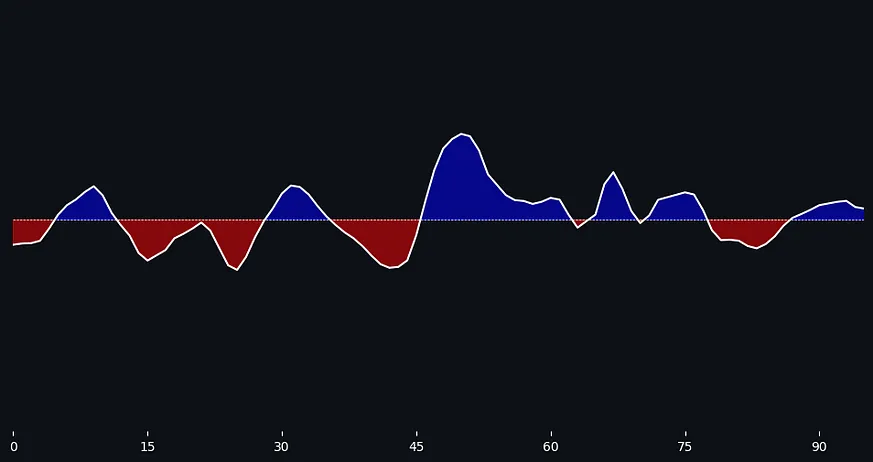
Next, we will label the teams, establish the axes, and set a title. Additionally, we are automatically calculating the scores using our primary data frame that contains event data.
scores = df[df['shot_outcome'] == 'Goal'].groupby('team')['shot_outcome'].count().reindex(set(df['team']), fill_value=0) ax.set_xlabel('Minute', color='white', fontsize=15, fontweight='bold', fontfamily='Monospace') ax.set_ylabel('Momentum', color='white', fontsize=15, fontweight='bold', fontfamily='Monospace') ax.set_title(f'xT Momentum\n{HOME_TEAM} {scores[HOME_TEAM]}-{scores[AWAY_TEAM]} {AWAY_TEAM}', color='white', fontsize=20, fontweight='bold', fontfamily='Monospace', pad=-5) home_team_text = ax.text(7, 0.064, HOME_TEAM, fontsize=12, ha='center', fontfamily="Monospace", fontweight='bold', color='white') home_team_text.set_bbox(dict(facecolor='blue', alpha=0.5, edgecolor='white', boxstyle='round')) away_team_text = ax.text(7, -0.064, AWAY_TEAM, fontsize=12, ha='center', fontfamily="Monospace", fontweight='bold', color='white') away_team_text.set_bbox(dict(facecolor='red', alpha=0.5, edgecolor='white', boxstyle='round'))
Let's include an additional detail – the specific minutes during which the goals were scored.
goals = df[df['shot_outcome']=='Goal'][['minute', 'team']] for _, row in goals.iterrows(): ymin, ymax = (0.5, 0.8) if row['team'] == HOME_TEAM else (0.14, 0.5) ax.axvline(row['minute'], color='white', linestyle='--', linewidth=0.8, alpha=0.5, ymin=ymin, ymax=ymax) ax.scatter(row['minute'], (1 if row['team'] == HOME_TEAM else -1)*0.06, color='white', s=100, zorder=10, alpha=0.7) ax.text(row['minute']+0.1, (1 if row['team'] == HOME_TEAM else -1)*0.067, 'Goal', fontsize=10, ha='center', va='center', fontfamily="Monospace", color='white')Here, I provide the complete code encapsulated within a single function:
from statsbombpy import sb import pandas as pd import numpy as np import matplotlib.pyplot as plt from scipy.ndimage import gaussian_filter1d def momentum(match_id, window_size=4, decay_rate=0.25, sigma=1): df = sb.events(match_id=match_id) HOME_TEAM, AWAY_TEAM= list(df['team'].unique()) xT = pd.read_csv("https://raw.githubusercontent.com/AKapich/WorldCup_App/main/app/xT_Grid.csv", header=None) xT = np.array(xT) xT_rows, xT_cols = xT.shape def get_xT(df, event_type): df = df[df['type']==event_type] df['x'], df['y'] = zip(*df['location']) df['end_x'], df['end_y'] = zip(*df[f'{event_type.lower()}_end_location']) df[f'start_x_bin'] = pd.cut(df['x'], bins=xT_cols, labels=False) df[f'start_y_bin'] = pd.cut(df['y'], bins=xT_rows, labels=False) df[f'end_x_bin'] = pd.cut(df['end_x'], bins=xT_cols, labels=False) df[f'end_y_bin'] = pd.cut(df['end_x'], bins=xT_rows, labels=False) df['start_zone_value'] = df[[f'start_x_bin', f'start_y_bin']].apply(lambda z: xT[z[1]][z[0]], axis=1) df['end_zone_value'] = df[[f'end_x_bin', f'end_y_bin']].apply(lambda z: xT[z[1]][z[0]], axis=1) df['xT'] = df['end_zone_value']-df['start_zone_value'] return df[['xT', 'minute', 'second', 'team', 'type']] xT_data = pd.concat([get_xT(df=df, event_type='Pass'), get_xT(df=df, event_type='Carry')], axis=0) xT_data['xT_clipped'] = np.clip(xT_data['xT'], 0, 0.1) max_xT_per_minute = xT_data.groupby(['team', 'minute'])['xT_clipped'].max().reset_index() minutes = sorted(xT_data['minute'].unique()) weighted_xT_sum = {team: [] for team in max_xT_per_minute['team'].unique()} momentum = [] for current_minute in minutes: for team in weighted_xT_sum: recent_xT_values = max_xT_per_minute[(max_xT_per_minute['team'] == team) & (max_xT_per_minute['minute'] <= current_minute) & (max_xT_per_minute['minute'] > current_minute - window_size)] weights = np.exp(-decay_rate * (current_minute - recent_xT_values['minute'].values)) weighted_sum = np.sum(weights * recent_xT_values['xT_clipped'].values) weighted_xT_sum[team].append(weighted_sum) momentum.append(weighted_xT_sum[HOME_TEAM][-1] - weighted_xT_sum[AWAY_TEAM][-1]) momentum_df = pd.DataFrame({ 'minute': minutes, 'momentum': momentum }) fig, ax = plt.subplots(figsize=(12, 6)) fig.set_facecolor('#0e1117') ax.set_facecolor('#0e1117') ax.tick_params(axis='x', colors='white') ax.tick_params(axis='y', which='both', left=False, right=False, labelleft=False) for spine in ['top', 'right', 'bottom', 'left']: ax.spines[spine].set_visible(False) ax.set_xticks([0,15,30,45,60,75,90]) ax.margins(x=0) ax.set_ylim(-0.08, 0.08) momentum_df['smoothed_momentum'] = gaussian_filter1d(momentum_df['momentum'], sigma=sigma) ax.plot(momentum_df['minute'], momentum_df['smoothed_momentum'], color='white') ax.axhline(0, color='white', linestyle='--', linewidth=0.5) ax.fill_between(momentum_df['minute'], momentum_df['smoothed_momentum'], where=(momentum_df['smoothed_momentum'] > 0), color='blue', alpha=0.5, interpolate=True) ax.fill_between(momentum_df['minute'], momentum_df['smoothed_momentum'], where=(momentum_df['smoothed_momentum'] < 0), color='red', alpha=0.5, interpolate=True) scores = df[df['shot_outcome'] == 'Goal'].groupby('team')['shot_outcome'].count().reindex(set(df['team']), fill_value=0) ax.set_xlabel('Minute', color='white', fontsize=15, fontweight='bold', fontfamily='Monospace') ax.set_ylabel('Momentum', color='white', fontsize=15, fontweight='bold', fontfamily='Monospace') ax.set_title(f'xT Momentum\n{HOME_TEAM} {scores[HOME_TEAM]}-{scores[AWAY_TEAM]} {AWAY_TEAM}', color='white', fontsize=20, fontweight='bold', fontfamily='Monospace', pad=-5) home_team_text = ax.text(7, 0.064, HOME_TEAM, fontsize=12, ha='center', fontfamily="Monospace", fontweight='bold', color='white') home_team_text.set_bbox(dict(facecolor='blue', alpha=0.5, edgecolor='white', boxstyle='round')) away_team_text = ax.text(7, -0.064, AWAY_TEAM, fontsize=12, ha='center', fontfamily="Monospace", fontweight='bold', color='white') away_team_text.set_bbox(dict(facecolor='red', alpha=0.5, edgecolor='white', boxstyle='round')) goals = df[df['shot_outcome']=='Goal'][['minute', 'team']] for _, row in goals.iterrows(): ymin, ymax = (0.5, 0.8) if row['team'] == HOME_TEAM else (0.14, 0.5) ax.axvline(row['minute'], color='white', linestyle='--', linewidth=0.8, alpha=0.5, ymin=ymin, ymax=ymax) ax.scatter(row['minute'], (1 if row['team'] == HOME_TEAM else -1)*0.06, color='white', s=100, zorder=10, alpha=0.7) ax.text(row['minute']+0.1, (1 if row['team'] == HOME_TEAM else -1)*0.067, 'Goal', fontsize=10, ha='center', va='center', fontfamily="Monospace", color='white')Thank you for taking the time to read my article. I would be grateful for any thoughts or recommendations you may have. If you're interested in more football-related content, feel free to check out my Twitter/X account.
References
Event data
Event data may refer to: Events within an Event-driven architecture; Events handled by Event stream processing; Events handled by Complex event processing ...
Source: WikipediaWhat is the difference between event data and display data?
Event data are the instantaneous values recorded at each scan interval. Display data are the maximum and minimum sampled values recorded within the display ...
Source: Yokogawa ElectricWhat is Event Data?
Event Data is a collection of time-stamped data points that capture important occurrences, actions, or changes within a system or application.
Source: DremioEVENTdata
Big-data Management. Our data analytics and reporting methods provide you with a valuable tool to assess your event. We are obsessed with accuracy and security!
Source: eventdata.grWhat is Event Data, And How Do You Use It? - Just Understanding Data
Event data describes anything that can be measured, tracked or recorded in some way. This post investigates the purpose of event data for businesses.
Source: understandingdata.comEvent Data | The Who, What, Why, and How of Event Data
Event data is a type of data that is collected and stored by various tracking tools or methods in order to provide insights about user behavior, traffic ...
Source: Ninetailedevent.data | jQuery API Documentation
Description: An optional object of data passed to an event method when the current executing handler is bound. version added: 1.1event ...
Source: jQuery API DocumentationEvent Data
The Event Data API provides raw data about events alongside context: how and where each event was collected.
Source: Crossref
 ALL
ALL sports
Discussions